


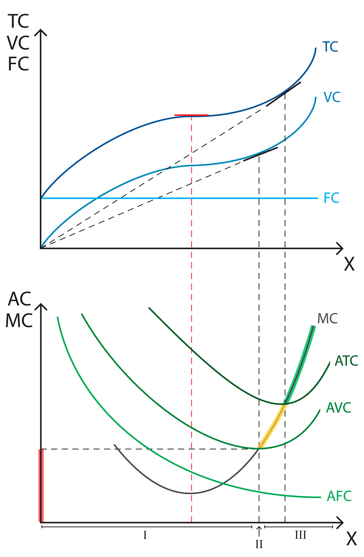
 In the short run, fixed costs include capital, K, whereas labour, L, is considered variable. Fixed costs are represented as a horizontal line and do not vary whatever level of production we achieve.
The two graphs show how the two phases pan out. In the first phase (I), variable costs (and therefore total costs, seeing as fixed costs are a constant) grow slower than growth at first, before reaching a point of inflection (II) and beginning to grow much faster than the output they are capable of generating.
This is related with returns to scale. In phase I, where the elasticity of scale is greater than 1, there are increasing returns to scale, while phase III corresponds to decreasing returns to scale. In point II, the elasticity of scale equals 1, which represents constant returns to scale.
If we translate this into average and marginal costs, an optimal level is reached along the stretch between which marginal costs are equal to average variable and fixed costs respectively. This coincides with the stretch just before costs begin to grow exponentially.