


Production in the very long run differs from long run production in that there may be changes in technology. There are three main types of technological advances:
- New technology allows for completely new products
- New technology allows us to produce equal quantities with less inputs, displacing our isoquants
- New technology allows us to produce greater quantities with equal inputs, displacing our production function
These technological advances may displace our ratio of capital to labour one way or the other. Let’s see it graphically first:
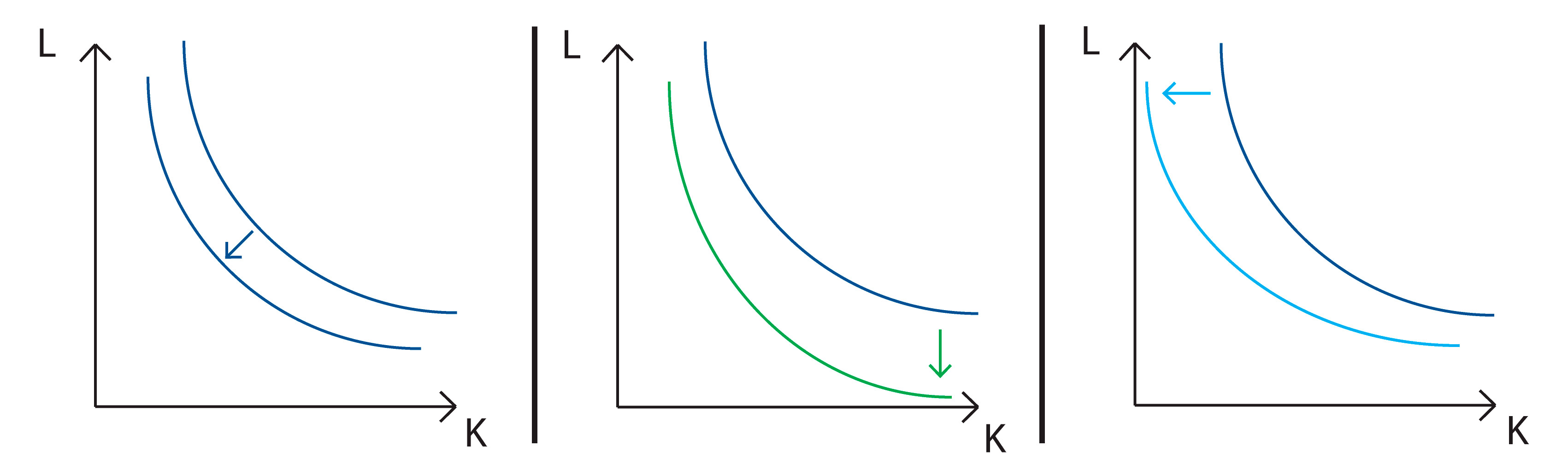
-the first technological change shown in the adjacent figure is called Hicks-neutral, which translates into an unchanged ratio of capital’s marginal product to labour’s marginal product. John Hicks devised it in his book “The Theory of Wages”, 1932. Analytically: Y = AF(K,L)
-the second technological change is called Harrod-neutral or labour-augmenting increases efficiency of labour. Roy Harrodformulated it in his book “Towards a Dynamic Economics”, 1948. Analytically: Y = F(K,AL)
-the third and last technological change shown is called Solow-neutral or capital-augmenting , which increases the efficiency of capital. It was devised by Robert Solow in his article “Technical Change and the Aggregate Production Function”, 1957. Analytically: Y = F(AK,L)
Finally, we must also take into account the possibility of endogenous growth derived from endogenous technical changes. This can be easily plotted by using a Cobb-Douglas function, such as:
